Digital operations on quantum computers

This is the third in a series of four articles based on my Jupyter Notebooks exploring quantum computing as a tool for generating random number distributions.

Generating random numbers from a variety of specific probability distributions shows us how the quantum state vector reflects the desired probability distribution, and the previous article showed how a variety of such distributions could be achieved. However, quantum computers can simulate a digital computer also. Even though bits are certain and qubits are uncertain, computing on a digital computer can be thought of like working with a special kind of probability distribution: one where there is a row on the state vector with a 100% probability, and all the rest are zero. This reflects how digital computers are deterministic.

Let’s look at how we might perform digital computing operations on a quantum computer, sticking with high-school level maths. First, we need to introduce some new operations.

X operation

We have already seen the CX, or “constrained swap”, operation. There is a simpler one called the X operation which does a swap within all pairs of rows in the state vector where the only difference is in a specific qubit. So, where the CX operation required specifying two qubits to determine the rows it affects, the X operation requires specifying just one qubit. Where you might think of CX as a “constrained swap”, you can think of X as just a “swap”.

To clarify the X operation, here is an example of how it might be used:

QubitsInitial state vectorX(0)X(1)
|00>1.00.00.0
|01>0.01.00.0
|10>0.00.00.0
|11>0.00.01.0

The first X swaps the first two rows, as these differ only in qubit 0 (the rightmost qubit), and while it also swaps the second two rows, these were the same, so we don’t see a difference there. The second X swaps rows |01> and |11>, as these differ only in qubit 1 (the leftmost qubit), and while it also swaps the remaining two rows, again these were the same value, so we don’t see any difference after the operation.

CCX operation

Now that we know about X and CX, you might be wondering if there are more constraints that can be added to X. Yes, a common operation is a “doubly constrained” version of X, sometimes known as a Toffoli operation.

The CCX operation is constrained to operate only on pairs of rows where two specified qubits are |1>, and it swaps pairs of rows where only a third qubit changes, i.e. a “doubly constrained swap” operation. Here’s what some CCX operations look like on a state vector consisting of three qubits:

QubitsInitial state vectorX(1)CCX(0, 1, 2)X(0)CCX(0, 1, 2)
|000> (|0>)1.00.00.00.00.0
|001> (|1>)0.00.00.00.00.0
|010> (|2>)0.01.01.00.00.0
|011> (|3>)0.00.00.01.00.0
|100> (|4>)0.00.00.00.00.0
|101> (|5>)0.00.00.00.00.0
|110> (|6>)0.00.00.00.00.0
|111> (|7>)0.00.00.00.01.0

Since our examples use Qiskit, qubits are numbered from the right. Qubit 0 is the rightmost one, then qubit 1 is in the middle, and qubit 2 is the leftmost one. In the above table, as it is starting to get long, next to the qubits identifier for the row, I’ve also written the row number in brackets. The qubits identifier is a binary number, and corresponds to a decimal number, which is the row number, e.g. “011” is the binary number for 3, so I’ve written this as |011> (|3>).

In this example, the CCX(0, 1, 2) operation swaps rows where qubits 0 (rightmost) and 1 (middle) are |1>, i.e. those rows ending in |11>: rows |3> and |7>. The first time this operation is performed, both of those rows are 0.0, so it looks like nothing happens, but the second time, we see the effect of the swap performed.

Incrementing a 3-bit number

A very common operation on a digital computer is incrementing a number, or in other words, adding one to it. Incrementing 3 results in 4, incrementing 6 results in 7, and so on.

Each row of the state vector represents a different number, i.e. the decimal number corresponding to the binary number for that arrangement of qubits. For a state vector that represents 3 qubits, row |100> is row |4>, while row |110> is row |6>. Incrementing a number can be thought of as taking a state vector with a specific number encoded in it – the row with 100% probability – and turning it into a state vector with a new number encoded in it, specifically the original number plus one. For example, if we start with a state vector with row |4> with 100% probability, incrementing this would result in a new state vector with row |5> having 100% probability.

To implement this sort of algorithm, where a row has 100% probability, and we make another row 100% probability, we simply need to use variants of the X operation. The X, CX and CCX operations only swap rows around, so will always leave the state vector having a single row with 100% probability. In this case, they can simulate the deterministic operations of a digital computer.

To increment a number encoded on the state vector using variants of the X operation, it is quite straightforward, but we need to think about it in binary notation. If we add one to a number ending in |0>, it becomes |1>. While if we add one to a number ending in |1>, it will become |0> and carry a one to the next place. To achieve this, we can use X to swap from a row |0> to a |1> row, or visa versa, and a CX to manage the carrying of the one. Similarly, we can use a CCX to manage the carrying of the one to the final place.

Implementing in Qiskit

Let’s create this increment operation as a Python function. (You can grab the complete Python script from here, or just type in the code below.)

import numpy as np
from qiskit import QuantumCircuit, QuantumRegister, ClassicalRegister
from qiskit.quantum_info import Statevector

# Add the operations to an algorithm that increments the number 
# encoded on a 3 qubit state vector
def add_increment(algo):
    algo.ccx(0, 1, 2) # Carry the one to qubit 2, when qubits 0 and 1 are |11>
    algo.cx(0, 1)     # Carry the one to qubit 1, when qubit 0 is |1>
    algo.x(0)         # Add one to qubit 0

Now we can test it out.

q = QuantumRegister(3)    # We want 3 qubits
algo1 = QuantumCircuit(q) # Construct an algorithm on a quantum computer

# Start in the |2> row
algo1.x(1)
v1 = Statevector(algo1)
print(np.real_if_close(v1.data))

$$\begin{bmatrix}
0.0 \\
0.0 \\
1.0 \\
0.0 \\
0.0 \\
0.0 \\
0.0 \\
0.0
\end{bmatrix}$$

# Increment the number encoded in the state vector
add_increment(algo1)
v2 = Statevector(algo1)
print(np.real_if_close(v2.data))

$$\begin{bmatrix}
0.0 \\
0.0 \\
0.0 \\
1.0 \\
0.0 \\
0.0 \\
0.0 \\
0.0
\end{bmatrix}$$

# Increment the number once more
add_increment(algo1)
v3 = Statevector(algo1)
print(np.real_if_close(v3.data))

$$\begin{bmatrix}
0.0 \\
0.0 \\
0.0 \\
0.0 \\
1.0 \\
0.0 \\
0.0 \\
0.0
\end{bmatrix}$$

We are successfully incrementing the number encoded in the state vector each time.

Doing multiple increments simultaneously

What if multiple numbers were encoded in the state vector? Actually, the same algorithm will continue to work.

Let’s start by encoding two numbers, so rather than one row having a 100% probability, the state vector will have two rows each with 1/√2 . Remember that we square this to get the probability, which will be 1/2 or 50%.

In Qiskit, we will encode both |0> and |3>, and apply the increment operation.

algo2 = QuantumCircuit(q) # Construct an algorithm on a quantum computer

# Start with |0> and |3> rows having equal probability
algo2.h(2)
v4 = Statevector(algo2)
print(np.real_if_close(v4.data))

$$\begin{bmatrix}
\frac{1}{\sqrt{2}} \\
0.0 \\
0.0 \\
0.0 \\
\frac{1}{\sqrt{2}} \\
0.0 \\
0.0 \\
0.0
\end{bmatrix}$$

# Increment the numbers encoded in the state vector
add_increment(algo2)

v5 = Statevector(algo2)
print(np.real_if_close(v5.data))

$$\begin{bmatrix}
0.0 \\
\frac{1}{\sqrt{2}} \\
0.0 \\
0.0 \\
0.0 \\
\frac{1}{\sqrt{2}} \\
0.0 \\
0.0
\end{bmatrix}$$

Now it has rows |1> and |4> with equal probability. Two increments have been performed simultaneously, without changing the increment operation at all. (In fact, the increment operation can also be thought of as a rotation operation, where the values are rotated through all of the rows of state vector, a row at a time.)

It is this sort of capability that highlights the power of quantum computers to rapidly speed up some types of computation.

In conclusion

We have added another two more operations to our set, and seen how to use them on a quantum computer to perform a traditional digital computer functions (incrementing a number). We’ve also seen how quantum computers can enhance digital functions, like performing multiple increments at once. Here is the set of operations we’ve talked about so far:

OperationShort-hand descriptionSpecified byDetailed description
H“half”1 qubitFor all pairs of rows that differ only by the value of a specific qubit in the outcome, replace the first row value with a new value that is the sum of the original values divided by √2, and the second row value with the difference between the original values divided by √2.
CX“constrained swap”2 qubitsFor all pairs of rows where the first qubit specified is in the |1> state in the outcome, and where otherwise the rows differ only by the value of the second qubit specified, swap the rows in the pair.
RY“relative swap”1 angle and 1 qubitFor all pairs of rows that differ only by the value of a specific qubit in the outcome, swap a fraction “f” of the value from the first row to the second, and bring the opposite fraction (i.e. 1-f) from the second row but with the sign flipped, where “f” is specified as the angle 2 x arcsin(√f). If “f” is 1.0, the angle will be 𝜋.
X“swap”1 qubitFor all pairs of rows that differ only by the value of a specific qubit in the outcome, swap the values in the pair.
CCX“doubly constrained swap”3 qubitsFor all pairs of rows where both the first and second qubit specified are in the |1⟩ state in the outcome, and where otherwise the rows differ only by the value of the third qubit specific, swap the rows in the pair

The next article will look at a well-known algorithm that performs a task that is complex on a digital computer but is very efficient on a quantum computer.
Further adventures in quantum randomness

This is the second in a series of four articles based on my Jupyter Notebooks exploring quantum computing as a tool for generating random number distributions.

The first article showed how a quantum computer could be programmed to generate a uniform random distribution of two bits using operations on qubits. It was a pretty trivial algorithm, and compared with the complexity of generating pseudo-random numbers on a digital computer, showed the advantage of using quantum computers for this application. However, given that I discussed how quantum computers can manipulate probabilities, it’s natural to consider how other, non-uniform, random number distributions might be calculated using a quantum computer. As with the first article, I’m sticking with high-school level maths.
Bell state

A special type of quantum state is known as the Bell state. There are actually four Bell states, but for simplicity, we’ll just pick one. To put a two qubit quantum computer into a Bell state, we will manipulate it to have the state vector

$$\begin{bmatrix}
\frac{1}{\sqrt{2}} \\
0.0 \\
0.0 \\
\frac{1}{\sqrt{2}}
\end{bmatrix}$$

which means that a measurement will get either the |00> or |11> outcomes with equal probability, but the |01> and |10> outcomes won’t appear at all. Another way to think of this is flipping two coins, and having them always end up heads-heads or tails-tails, but never getting a heads-tails result.

To get this state vector, it’s not enough to use the H operation, but we need something called the CX operation.

CX operation

The CX operation can be thought of as a “constrained swap” operation which affects pairs of rows in the state vector specified by the states of two qubits (rather than specified by just one qubit, like we saw with the H operation). It will cause the values of those pairs of rows to swap, constrained to those pairs of possible outcomes where the first qubit specified is in the |1> state and that otherwise differ only by the value of the second qubit.

For example, if we start with the usual initial state vector for two qubits:

QubitsInitial state vector
|00>1.0
|01>0.0
|10>0.0
|11>0.0

where the |00> outcome has a 100% probability, and now apply the CX operation against the right-most qubit then the left-most qubit, or CX(0,1) to use the Qiskit numbering for qubits, the state vector wouldn’t change at all, since the pair of rows where the right-most qubit is |1> are both the same, i.e. 0.0, so swapping doesn’t change anything.

However, if we firstly use the H operator on rows associated with the right-most qubit, or an H(0) operation, and then perform the same CX(0,1) operation, we get a more interesting result:

QubitsInitial state vectorWorking out H(0)Result of H(0)Working out CX(0,1)Result of CX(0,1)
|00>1.0=(1.0+0.0)/√21/√2unchanged1/√2
|01>0.0=(1.0-0.0)/√21/√2=0.00.0
|10>0.0=(0.0+0.0)/√20.0unchanged0.0
|11>0.0=(0.0-0.0)/√20.0=1/√21/√2

Swapping the rows made a change this time, and we have ended up with the Bell state that we were talking about above.

Implementing this on Qiskit

Now, let’s create a histogram of the results we get from performing this on a (simulated) quantum computer, and check that it does what we expect. We’ll use the same approach with Qiskit as we did last time. (You can grab the complete Python script from here, or just type in the code below.)

import numpy as np
from qiskit import QuantumCircuit, QuantumRegister, ClassicalRegister, execute, BasicAer
from qiskit.visualization import plot_histogram
import matplotlib.pyplot as plt
backend = BasicAer.get_backend('qasm_simulator')

q = QuantumRegister(2)   # We want to use 2 qubits
algo = QuantumCircuit(q) # Readies us to construct an algorithm to run on the quantum computer

algo.h(0)          # Apply H operation on pairs of rows related to qubit 0
algo.cx(0,1)       # Apply CX operation, constrained where qubit 0 is |1>
algo.measure_all() # Measure the qubits and get some bits

result = execute(algo, backend, shots=1000).result()
plot_histogram(result.get_counts(algo))
plt.show()

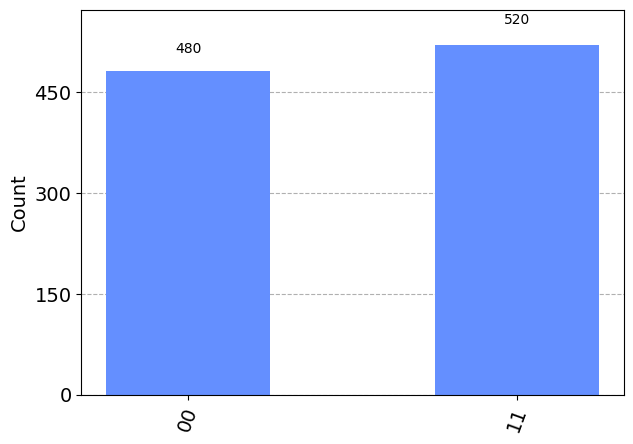
Yes, this is the random distribution we were hoping to get. It is just “00” and “11” with no “01” or “10” results.

RY operation

We’ve achieved a non-uniform distribution, but it’s not a very interesting one. It’s a 50-50 outcome, and we could have achieved that with 1 qubit. We didn’t really need 2 qubits. To create more interesting distributions, we will need another operation. Let’s take a look at the RY operation.

RY adjusts the pairs of state vector rows applying to a specified qubit, and adjusts them by a specified “angle”. If the angle is pi (𝜋), which is an amount in radians equivalent to 180 degrees, the adjustment results in a swap of values and flipping the sign of the first value (we’ll come back to this). But the swap is modified relative to the angle, so we can think of it like a “relative swap” operation.

Let’s have a look at at how it would work on the standard initial state vector, with the specific qubit being the right-most one (or, qubit 0), and for some different angles:

QubitsInitial state vectorR(0.0, 0)R(𝜋, 0)R(𝜋, 0) againR(𝜋/2, 0)
|00>1.01.00.0-1.0-1/√2
|01>0.00.01.00.0-1/√2
|10>0.00.00.00.00.0
|11>0.00.00.00.00.0

The first time the RY operation is used, it is given a specified angle of 0.0, and it does absolutely nothing to the state vector. This is correct – with an angle of 0.0, RY will not change anything.

Next, we can see that when the RY(𝜋, 0) operation happens, it swaps the values where the right-most qubit (qubit 0) differ, i.e. the first and second row, and the third and fourth row. In addition, it flips the sign on the first of each pair of rows. The first time RY happens, it simply moves the 100% outcome from |00> to |01>. The second time RY happens, it moves this outcome back to |00> and flips the sign to negative.

What does -100% mean? How can this be a probability? Well, each row of the state vector is a probability amplitude rather than a probability. If a probability amplitude is a real number, i.e. no imaginary component, you can turn it into its corresponding probability by just squaring it. -1.0 x -1.0 is 1.0, so -100% as a probability amplitude is equivalent to a 100% probability. Note that this isn’t just some oddity, but actually part of what makes quantum computers powerful.

The final application of the RY operation in the table is with a specified angle that is 𝜋/2 which corresponds to 90 degrees. It’s mid-way between 0.0 and 𝜋, and produces a result that is also mid-way between the previous results. Where the 0.0 angle didn’t move any of the probability amplitude values between the pairs, and the 𝜋 angle moved all of the probability amplitude values to the alternate row in each pair, the 𝜋/2 angle is halfway between those angles and it moved half the probability amplitude, in the same way the H operator did in the previous notebook.

In fact, we can pick an angle to give to the RY operation that will move a desired fraction of the probability amplitude value between the rows. To swap a fraction “f” of the value from the first row to the second, and bring the opposite fraction (i.e. 1-f) from the second row but with the sign flipped, you use the angle calculated by 2 x arcsin(√f). For our final application of RY above, it had the fraction f=1/2, and it turns out that 2 x arcsin(√(1/2)) = 𝜋/2 which is the angle used in the operation.

We can now use this knowledge to create a range of specific probability distributions for our random bits. The set of operations we have talked about so far – H, CX and RY – should allow us to create any probability distribution. For example, if we want to create a probability distribution where it is equally likely that any of the first three outcomes (|00>, |01>, and |10>) happen and yet the last outcome (|11>) shouldn’t happen, the state vector we’d want to create is:

$$\begin{bmatrix}
\sqrt{\frac{1}{3}} \\
0.0
\end{bmatrix}$$

A way to get this is to recognise that if we look at the state vector as two pairs of rows, the first pair of outcomes are twice as likely in total as the second pair of outcomes. We can use the RY operation to swap (the square root) of a third of the overall probability to the second pair. We can then use a sequence of H, RY, CX and RY operations to spread the probabilities within each pair. This looks like:

QubitsInitial state vectorRY(2 x arcsin(√(1/3)), 1)H(0)RY(𝜋/4, 0)CX(1, 0)RY(-𝜋/4, 0)
|00>1.0√(2/3)√(1/3)0.31250.3125√(1/3)
|01>0.00.0√(1/3)0.75430.7543√(1/3)
|10>0.0√(1/3)√(1/6)0.22090.5334√(1/3)
|11>0.00.0√(1/6)0.53340.22090.0

You can see here that after the H(0) operation, the first two rows have the values we want, but the final two rows had the desired values before the H(0). The operations following the H(0) have the effect of undoing the H(0) operation on the final two rows but leaving the first two rows alone. Note that the final two RY operations are opposite signs to each other, so they should cancel each other out, but a CX(1,0) operation has been done in the middle. This CX operation, in swapping the final two rows, has the effect of making it as if the first of the final two RY operations was also a negative angle for those rows, so instead of cancelling out (like happened on the first two rows), the two RY operations on those rows add together as if it was an RY operation of -𝜋/2. As we saw above, an RY operation with the angle 𝜋/2 is similar to an H operation, and with the negative angle, the RY operation acts to reverse the H.

Don’t worry if you didn’t fully follow that. This sort of procedure is called “amplitude embedding” or “state preparation”, and there are various algorithms to do this, many of which get quite esoteric. The above procedure was inspired by a paper by Mottonen, Vartiainen, Bergholm, and Salomaa. The main thing to note is that quantum computers allow arbitrary non-uniform distributions to be constructed.

Implementing this on Qiskit

Let’s test the above procedure and see if it does what we expect. (You can grab the complete Python script from here, or just type in the code below.)

import numpy as np
from qiskit import QuantumCircuit, QuantumRegister, ClassicalRegister, execute, BasicAer
from qiskit.visualization import plot_histogram
import matplotlib.pyplot as plt
backend = BasicAer.get_backend('qasm_simulator')

q = QuantumRegister(2)   # We want to use 2 qubits

angle1 = 2 * np.arcsin(np.sqrt(1.0/3.0))
angle2 = np.pi / 4

algo = QuantumCircuit(q) # Readies us to construct an algorithm to run on the quantum computer

algo.ry(angle1, 1)       # Apply RY operation to swap 1/3 of qubit 1's value 
algo.h(0)                # Apply H operation on pairs of rows related to qubit 0
algo.ry(angle2, 0)       # Apply RY operation to perform a half of H on qubit 0
algo.cx(1,0)             # Apply CX operation, constrained to where qubit 1=|1>
algo.ry(-angle2, 0)      # Apply RY operation to undoing half of H on qubit 0

algo.measure_all()       # Measure the qubits and get some bits

result = execute(algo, backend, shots=1000).result()
plot_histogram(result.get_counts(algo))              
plt.show()

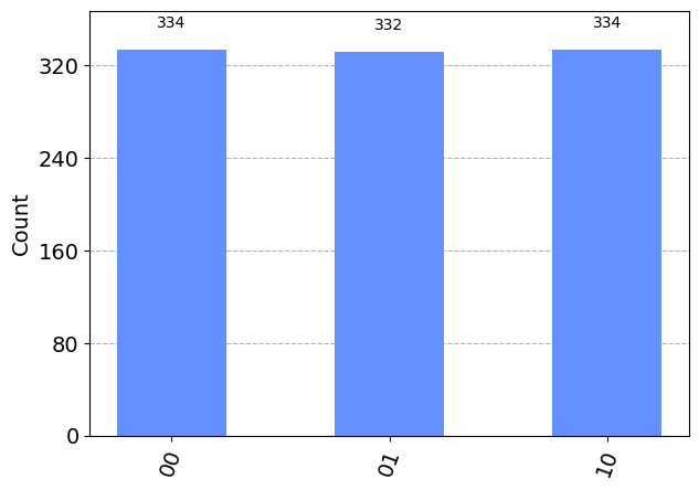
This is exactly what we were hoping to see. It is “00”, “01” and “10” split three ways, and with no “11” results.

In conclusion

We have added two more operations to our set, and seen how to use them on a quantum computer to create a variety of random distributions, such as the Bell state:

OperationShort-hand descriptionSpecified byDetailed description
H“half”1 qubitFor all pairs of rows that differ only by the value of a specific qubit in the outcome, replace the first row value with a new value that is the sum of the original values divided by √2, and the second row value with the difference between the original values divided by √2.
CX“constrained swap”2 qubitsFor all pairs of rows where the first qubit specified is in the |1> state in the outcome, and where otherwise the rows differ only by the value of the second qubit specified, swap the rows in the pair.
RY“relative swap”1 angle and 1 qubitFor all pairs of rows that differ only by the value of a specific qubit in the outcome, swap a fraction “f” of the value from the first row to the second, and bring the opposite fraction (i.e. 1-f) from the second row but with the sign flipped, where “f” is specified as the angle 2 x arcsin(√f). If “f” is 1.0, the angle will be 𝜋.

The next article will look at how to implement digital computing functions through operations on the state vector.

A Quantum Computer is a random number generator

This is the first in a series of four articles based on my Jupyter Notebooks exploring quantum computing as a tool for generating random number distributions.

Many of the introductory quantum computing articles and courses out there are not quite right. They either quickly head deep into details that require a University-level physics or mathematics background, or sit at a high level based on analogies that are out of step with how quantum computers actually work. I want to try something different, and introduce some useful quantum computing algorithms using high-school level maths. I will avoid much (but maybe not all) of the jargon, and show how the algorithms can be implemented on the commonly available Qiskit platform.

In my earlier article on quantum computing, I introduced an analogy to describe quantum computers, which are based on qubits rather than bits. The analogy was of a coin-flipping robot arm that is flipping a coin that lands on a table. A qubit is like the coin when it is in the air, and a bit is like the coin when it has ended up on the table. When it’s in the air, the coin is in a kind of probabilistic state where it may end up heads or tails, but once it’s on the table, it’s in a certain state where it is definitely one of either heads or tails. Quantum computers work in the realm of probabilities, and can manipulate the coin while it’s still spinning in the air. The spinning coin in the air is the qubit. But at some point it will land on the table and be measured as either heads or tails. At that point it becomes a bit.

To write about quantum states, a notation is used where the name of the state is put between a vertical bar and an angle bracket. Just like a single bit can be in the “0” state or the “1” state, for a single qubit, we might say it can be in the |0> state or the |1> state. Our hypothetical robot-arm is well-calibrated, so it consistently flips a coin that lands with the same side facing up, and the resulting coin is like having a qubit in one of these states. The coin is in a probabilistic state, but the probability of it having a particular result is 100%. Similarly, if a qubit is in the |0> state, when it is measured, you will get a “0” result 100% of the time.

However, a quantum computer can manipulate the probabilities of the qubit, so even if the qubit started in the |0> state, after manipulation it enters a new state where if the qubit is measured, it will get “0” outcome 50% of the time (and “1” outcome the other 50% of the time, of course). This is done using a Hadamard operation, usually just written as H. We will use this operation to create truly random numbers.

Creating truly random numbers

Mostly when you have a computer give you a random number, such as using the RAND function in Microsoft Excel or when you’re playing a computer game and the enemy does something unexpected, the computer is actually producing a pseudo-random number. If you could create a perfect snapshot of everything in your computer, then get it to do something “random”, and return to that snapshot again, it will do exactly the same random thing each time. So, it’s not actually random, but it looks random unless you peer too closely.

For most applications, that’s fine. But if you are doing cryptography, having truly random numbers is important. You want to generate a secret key that no-one else can guess. Ideally, even if someone could take a snapshot of your computer, they still couldn’t predict what secret key is generated. There are special hardware random number generators that can create truly random numbers (Cloudflare uses lava lamps!), and quantum computers create truly random numbers too.

Let’s say we are going to generate a 2 bit random number. We’ll use 2 qubits, and the starting state of the qubits will be |00>, which means the outcome of measuring them both as “0” is 100%. We’ll use a quantum computer to manipulate the qubits so that all four possible outcomes |00>, |01>, |10>, or |11> are equally likely. Then when the qubits are measured, we will have some truly random bits.

We can write the four possibilities as a vector, with each row consisting of the probability of that outcome. Quantum computers perform their calculations using complex numbers rather than real numbers, and this is because complex numbers are needed to accurately describe how things work at the quantum level. We can simplify things, and just use real numbers, but we will need to calculate probabilities by squaring the values in each row of the vector.

We call this vector the quantum state vector (or just state vector), and it starts with being

$$\begin{bmatrix}
1.0 \\
0.0 \\
0.0 \\
0.0
\end{bmatrix}$$

Each row of the state vector corresponds to a different outcome, with the outcomes for two qubits being |00>, |01>, |10>, and |11> as we go down the vector. So this state vector represents a 100% probability of getting the |00> outcome.

We want each outcome to have a 25% probability, so we want to change the state vector to be:

$$\begin{bmatrix}
\frac{1}{2} \\
\frac{1}{2} \\
\frac{1}{2} \\
\frac{1}{2}
\end{bmatrix}$$

Of course, when you square 1/2, you get 1/4, or 25%.

The H operation is a standard operation on quantum computers, and works on all pairs of rows of the quantum state vector where that outcome differs only by the value of a specific qubit, e.g. where one outcome has the |0> for that qubit and the other row has |1>. For each pair, it turns the first value into a new value that is the sum of the original values divided by \(\sqrt{2}\), and the second value into the difference between the original values divided by \(\sqrt{2}\). While it is a division by \(\sqrt{2}\) rather than a division by 2, you can think of H like a “half” operation, where it calculates half the sum and half the difference and is scaled by a normalisation constant so that when the values are squared, the probabilities add up to 1.0. Written out mathematically, if the first row value is \(a\) and the second row value is \(b\), the first row value becomes \(\frac{a+b}{\sqrt{2}}\) and the second row value becomes \(\frac{a-b}{\sqrt{2}}\).

To get the desired final state vector from the initial state vector, we can apply H first to the pair of rows associated with a difference in the right-most qubit, then apply H to the pair of rows associated with a difference in the left-most qubit. Here’s how it would go:

QubitsInitial state vectorWorking out first HResult of first HWorking out second HResult of second H
|00>1.0=\(\frac{1.0+0.0}{\sqrt{2}}\)\(\frac{1}{\sqrt{2}}\)=\(\frac{\frac{1}{\sqrt{2}}+0.0}{\sqrt{2}}\)\(\frac{1}{2}\)
|01>0.0=\(\frac{1.0-0.0}{\sqrt{2}}\)\(\frac{1}{\sqrt{2}}\)=\(\frac{\frac{1}{\sqrt{2}}-0.0}{\sqrt{2}}\)\(\frac{1}{2}\)
|10>0.0=\(\frac{0.0+0.0}{\sqrt{2}}\)0.0=\(\frac{\frac{1}{\sqrt{2}}+0.0}{\sqrt{2}}\)\(\frac{1}{2}\)
|11>0.0=\(\frac{0.0-0.0}{\sqrt{2}}\)0.0=\(\frac{\frac{1}{\sqrt{2}}-0.0}{\sqrt{2}}\)\(\frac{1}{2}\)

Now that we’ve covered the process, let’s look at how this would be written programmatically using the Qiskit library from IBM.

Implementing this on Qiskit

We’re going to set up a (simulated) quantum computer with 2 qubits. (You can grab the complete Python script from here, or just type in the code below.)

import numpy as np
from qiskit import QuantumCircuit, QuantumRegister, ClassicalRegister, execute, BasicAer
from qiskit.quantum_info import Statevector
from qiskit.visualization import plot_histogram
import matplotlib.pyplot as plt
backend = BasicAer.get_backend('qasm_simulator')

q = QuantumRegister(2)   # We want to use 2 qubits
algo = QuantumCircuit(q) # Readies us to construct an algorithm to run on the quantum computer

By convention, all qubits begin in the lowest-energy state, so without doing anything, the qubits of our quantum computer should be set to |00>. We can check the state vector and see.

v1 = Statevector(algo)
print(np.real_if_close(v1.data))

Which will print “[1. 0. 0. 0.]” and shows the |00> row is 1.0 and the other possible outcomes are 0.0.

Qiskit numbers the right-most qubit as qubit 0, and the one to the left of it as qubit 1, with the next as qubit 2, and so on. You may have come across this as being called little-endian. Let’s start by using the H operator on pairs of rows associated with the |0> and |1> outcomes on qubit 0 (the right-most qubit).

algo.h(0)  # Apply H operation on pairs of rows related to qubit 0
v2 = Statevector(algo)
print(np.real_if_close(v2.data))

Which will print “[0.70710678 0.70710678 0. 0. ]”, and given 0.70710678 is \(\frac{1}{\sqrt{2}}\), it is what we were expecting. Now to do the H operation on the pairs of rows associated with the other qubit (qubit 1).

algo.h(1)  # Apply H operation on pairs of rows related to qubit 1
v3 = Statevector(algo)
print(np.real_if_close(v3.data))

Which will print “[0.5 0.5 0.5 0.5]”. The application of the H operations has set up the state vector so that the quantum computer should give us different randomly generated 2 bit values with uniform distribution. Let’s add a measurement to the end of our algorithm, and have the quantum computer do this 1,000 times and see what we get.

algo.measure_all()  # Measure the qubits and get some bits
result = execute(algo, backend, shots=1000).result()  # Run this all 1,000 times
plot_histogram(result.get_counts(algo))
plt.show()
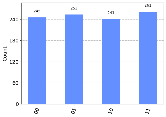
chart with four columns of similar height, labelled with 00, 01, 10 and 11

This shows that of the 1,000 times this was performed (1,000 “shots”), the different 2-bit results occurred approximately the same number of times. It is what you would expect of a uniform distribution, noting that it is unlikely for every possibility to occur exactly the same number of times.

You can extend this process to as many random bits as you want, by having a qubit for each and applying the H operation in turn for each qubit. Quantum computers are still not very big, so you’ll run out of available qubits quickly. Or, you may want to just to re-run this process and get another two random bits each time.

We used a quantum computer simulator here, so it’s still a pseudo-random result. To use an actual quantum computer, you would need to set up an account on IBM Quantum, get an API key, and change the backend to point at an instance of a quantum computer from their cloud. This is easy enough to do, but is an unnecessarily complication for this article.

You can then access true random bits that can be fed into any software that needs it. With all that, you have seen how to create a simple quantum algorithm and make it do something useful that is not easily done on a digital computer.

Please let me know… Were you able to follow this description of quantum computation? Do you feel confident that you could get this working on a real quantum computer? Would you prefer if there was more linear algebra, matrices and complex numbers in this article?

My main insight from SXSW Sydney

Last week, I attended the inaugural SXSW Sydney, and the first SXSW outside of Texas. It was different to the regular tech conferences that I’ve attended – it was much more diverse, with the games/film/music streams attracting a broader crowd. The sessions that I made it into were stimulating and sparked a range of ideas.

Of course, topics like AI (particularly Generative AI) and the Future of Work featured heavily in many presentations, and this led me to a realisation that I hadn’t had before, and I feel is likely to be the biggest impact from GenAI in the medium term. Rather than keep it to myself, I am sharing it here so that I can hear from others if it makes sense to them also.

Specifically, GenAI will bring about a huge disruption to the professional workforce and education system, not necessarily because humans will be replaced, but because humans who have been excluded from participation will now have fewer barriers to entry. Proficiency in the English language has been used as a justification for keeping certain people out of certain fields, and GenAI allows anyone from a non-English background to be as creative, smart, and persuasive as they are in their native tongues.

Our current GenAI systems are largely based on the Transformer machine learning architecture, which showed up early in online language translation tools like Google Translate. However, the GPT (T stands for Transformer) systems, particularly ChatGPT, have shown us that only a few words in broken English are able to be turned into paragraphs of words in perfect English, or even the reverse where paragraphs are summarised down to a few points in another language. University-level English spelling, grammar, and comprehension are no longer the exclusive domain of the English fluent.

There’s a fun TV series called Kim’s Convenience about a Korean couple who move to Canada to raise their family. The couple were teachers in Korea, but instead of doing that, they open a convenience store in Toronto. Presumably their lack of English or French language fluency would have been a limitation in getting teaching jobs. However, less than two months ago, OpenAI published their guide for teachers around ChatGPT, and it included the use case of “Reducing friction for non-English speakers”. In this guide, it was to help non-English students, but many of the suggestions could help non-English teachers also.

About 6% of the world’s population are native English speakers, and 75% do not speak English at all. And yet, about a third of the world’s GDP comes from countries where English fluency is required for success. If English is no longer a barrier to success in that market, it will be a significant disruption.

The spread of remote working technologies due to the pandemic has changed the ways of working for many jobs. Many white-collar jobs will likely still have an element of face-to-face contact, even if to come together for celebrations or training. However, where workers can be fully remote, the lack of English fluency as a barrier will enable many countries to export their talent without it leaving their shores.

Before the pandemic hit, over a quarter of University revenues in Australia came from international students. This gives international students some influence over University policies, and currently they face English language proficiency tests as part of their enrolment and visa processes. In the near future, GenAI looks set to be considered a generally-available tool in the workplace, like a calculator or laptop. If prospective students could make use of such a tool to address any gaps in their English language skills post-graduation, is it fair to prevent them from using it before graduation?

Traditionally, those people who had limited English in countries like Australia, UK or USA had been resigned to taking a jobs as an “unskilled” worker. There are already concerns that the number of people willing to do this type of work might not be enough to meet future industry demands. What might happen to wages if a good proportion of these people were able to move out of the unskilled workforce? How readily can the creative and information worker industries expand to take on new talent? What new barriers might be created by unions and professional organisations to help limit a flood of new workers into their industries?

GenAI has been making headlines that AI is taking many people’s creative jobs. After hearing from several panels at SXSW on AI, Long-term Forecasting, Work of the Future, and Education, my conclusion is that a plausible and perhaps more relevant headline would be that GenAI will allow many more people to take on creative jobs.

Why Indigenous Australians are special

In Australia, we are about to vote in a referendum to change the constitution, to add an “Aboriginal and Torres Straight Islander Voice” to the list of government entities. We’ll get to vote Yes or No on the 18th (oops, I mean 14th) October, and it will be the first time in over 20 years that we’ve had the opportunity to do something like that.

I’ve had many discussions with people here about the Voice, and I will probably vote Yes given there are a majority of Indigenous Australians who want it. The idea for it came out of the 2017 First Nations National Constitutional Convention, and had been preceded by many years of discussion of how to recognise Indigenous Australians in the constitution. The “Uluru Statement from the Heart” summarises the majority position of a large number of Elders from this convention, and includes the statement “We call for the establishment of a First Nations Voice enshrined in the Constitution”.

I am not going to present here an argument or evidence for why this should be supported. There are good analyses elsewhere. However, one of the things that has come up when I’ve discussed the Voice with others is that if the Voice is seen as a way of addressing disadvantage (which it is intended to be), and if Indigenous Australians are a significantly disadvantaged group (which they are), why should they get a Voice in the constitution in priority over other disadvantaged groups, e.g. refugees? Why should we call out a particular population in the constitution? In other words, why are Indigenous Australians special?

I may not be qualified to answer this. My school education in Australia was at a time when Indigenous Australians were not well covered in the curriculum. I do not have lived experience when it comes to Indigenous Australian communities. However, I have tried to educate myself. I’ve read all six books in the First Knowledges series, books by Stan Grant, Bruce Pascoe, and Bill Gammage, and even Indigenous Australia for Dummies. I have listened to the 2022 Boyer lectures by Noel Pearson, and I’ve visited many parts of Australia with Indigenous tour guides, and try to listen.

Despite that, I haven’t seen an answer to this question so far in the copious material flying around the Internet on the Voice referendum, and it seems central to the claim of the No case that the proposed constitutional change will create an unwelcome new division in our society, so I’m going to give this a crack.

A first response is that this question is an example of Whataboutism, and raising the disadvantage of other groups doesn’t somehow disprove the need for Indigenous Australians to get better outcomes than they’ve gotten historically. Additionally, presumably all groups should get the support they need to address their disadvantage. It’s not an either-or. We should do better. However, I’ll take on the question as if it was asked sincerely.

Another response is that the question is backwards. That it is instead Indigenous Australians that make Australia so special. The something-around 60,000 years of time spent shaping and learning about the flora, fauna and geography of this country has helped us be what we are today. After European settlement, the Indigenous people have played a role in making early settlers, explorers and farmers succeed. My grandmother was helped into the world by an Indigenous mid-wife, for example. While this is a valid response, I feel it doesn’t treat the question seriously.

I’ve come across two arguments for why First Australians are special enough to merit their own constitutionally-endorsed organisation: a legal one, and a moral one.

The legal one is essentially that they have unique rights that no-one else in Australia has, both recognised by the High Court and covered in Commonwealth legislation, but this uniqueness is ignored by the constitution. What is known as the Mabo Case was a claim of “native title” rights to the Murray Islands – part of the Torres Straight islands, off the coast of Queensland – by Eddie Mabo and others. This was due to the people there continuing their traditional activities since before European settlement, and recognition of the traditional laws and society that underpinned these. While no other population of people who have arrived in Australia since European settlement can claim this, it is not a unique situation internationally. For example, in Canada it is also recognised that Indigenous peoples there have rights that pre-existed any colonisation. Importantly, these rights don’t result simply from genetic lineage or “race”, but due to being part of a society that has continued to exist in Australia for thousands of years.

The moral one is Australian governments (both state and federal) have consistently passed laws to the detriment of Indigenous Australians, and are able to continue to do so because of an imbalance of power between the various governments in power and the Indigenous populations. Until Indigenous people have more say over what is done to them, the situation risks continuing. Some examples of Commonwealth government actions that targeted Indigenous Australians include:

Additionally, one legal expert has claimed that “Australia is the only industrialised nation that allows its parliament to make special detrimental laws for the Indigenous peoples of the land.” If so, Australia is not covering itself in glory here.

To guarantee a say about the stream of regular measures and laws that are targeted towards them by the Commonwealth government requires something that is not entirely subject to the Commonwealth government. Previous entities that represented Indigenous interests (NACC, ADC, and ATSIC) each managed to survive for a few years before being abolished by the Commonwealth. Having a new entity established by the constitution provides more balance and continuity in the relationship.

In conclusion, there is no new division here. Indigenous Australians are set apart from other Australians due to access to unique rights, and due to being uniquely and repeatedly targeted by Commonwealth government activities and laws. If the referendum succeeds, this will not change. But we can hope that other things change for the better.

Making a VRM avatar from Ready Player Me

When I went looking to create an avatar, I discovered that there were a lot of options. There are 2D avatars that look like animated illustrations and 3D avatars that look like video game characters. There are full-body avatars, and half-body avatars (the top half, if you’re wondering). There are avatars tied to a particular app or service, and avatars that use an interoperable standard. There are many standards.

I decided that I wanted a full-body 3D avatar, since this seems to be the way things are headed. If I was using a Windows PC, I would be able to use something like Animaze and have my avatar track to my gestures and expressions. However, I am currently using a Mac and there are fewer options, especially in English. I was able to find the browser-based FaceVTuber service and the application 3tene, though. 3tene requires avatars in the VRM standard, so that made my decision for me.

The easiest way to create a VRM avatar seems to be to use VRoid Studio application, although the resulting avatars look like anime characters. I wanted to create a more realistic looking 3D avatar, and a service like ReadyPlayer.Me would be perfect, as it quickly creates an avatar based on a photo. The catch is that ReadyPlayer.Me does not yet export a VRM file version of their avatars. But there is a way to do it, if you’re willing to jump through some hoops.

This is a guide that I’ve put together based on trial and error, and heavily inspired by ReadyPlayer.Me’s instructions on exporting to a GLB file for Unity and Mada Craiz’s video on converting a ReadyPlayer.Me GLB file into a VRM file.

Firstly, you will need to have downloaded Blender and Unity / Unity Hub. For Unity, you will probably need to also set up an account. This guide was based on using Blender v3.2.1 and Unity 2020.3.39f1 Intel.

You will also need to download the UniVRM package for Unity. I used v0.103.2, which was the latest version at the time. Make sure you download the file named something like UniVRM-0.xxx.x_xxx.unitypackage. You don’t need the other files.

How to create a VRM file from a Ready Player Me avatar

  1. Create a folder that you’re going to store all the avatar assets in, let’s call it vrm_assets.
  2. Create an account on ReadyPlayer.Me, and build an avatar for yourself. It’s pretty fun.
  3. Click on “My Avatars”. You may need to click on Enter Hub to see this menu option.
  4. Click on the 3-dots icon on your avatar, and select “Download avatar .glb”, and store it in vrm_assets (or whatever you called that folder before).
    screenshot of page within Ready Player Me showing the menu to download a GLB file
  5. Open Blender, and start a New File of the General type.
  6. In the Scene Collection menu, right-click the Collection and choose Delete Hierarchy, to get rid of everything in the scene.
  7. Then select File > Import > glTF 2.0 (.glb/.gltf) menu option, pick the avatar GLB file that you downloaded from ReadyPlayer.Me and stored in vrm_assets, and click “Import glTF 2.0”.
  8. If you’re worried that all of the colours and textures are missing, you can get them to appear by pressing “Z” and selecting Material preview, but you can skip this step.
  9. Select the Texture Paint on the top menu bar to enter the Texture Paint workspace.
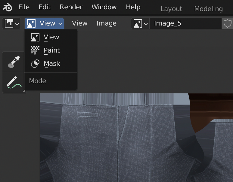
  10. Change the “Paint” mode to the “View” mode in the menu in the top left of the Texture Paint workspace screen.
    screenshot of Blender showing where the View menu is
  11. Then use the texture drop-down in the menu bar at the top to select each Image_0, Image_1, texture etc. in turn.
  12. For each texture, select the  Image > Save As menu option to save as individual images in your vrm_assets folder. Some of the textures could be JPG files while others are PNG files. Don’t worry about that. Just make sure you save all the images, but you can ignore “Viewer Node” or “Render Result”.
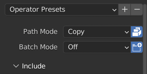
  13. Now select File > Export > FBX (.fbx) and before you save, change the “Path Mode” to “Copy” and click on the button next to it to “Embed Textures”. Then click the “Export FBX” button to save it into vrm_assets as well.
    Screenshot in Blender showing where to set Path Mode to Copy
  14. Close down Blender, and open up Unity Hub.
  15. Create a New Project, and select an Editor Version that begins 2020.3 and using the 3D Core template. Give the project a name that works for you, but I will use “VRM init”. Click “Create project”.
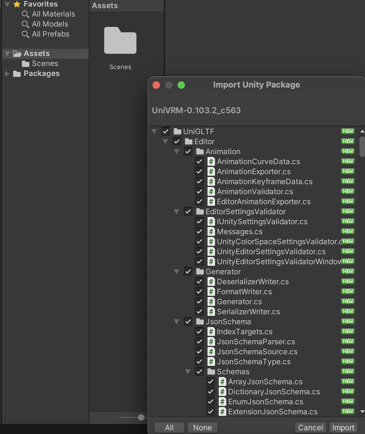
  16. Wait a little while for it to start up, then a blank project will appear. The first thing to do is bring in the UniVRM unitypackage file, so drag that from the file system into the Assets window. You will be shown an import window, with everything selected. Just click Import to bring it all in. After it’s done, UniGLTF, VRM and VRMShaders will be added to the Assets window.
    Screenshot of Blender showing the import of the unity package
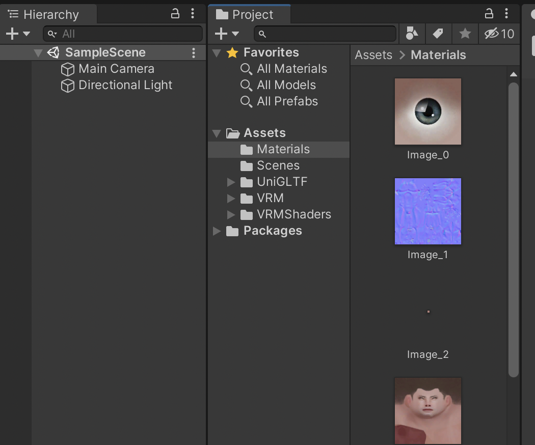
  17. Create a new folder in the Assets window called Materials. Open the Materials folder, then drag all the texture files from vrm_assets over into it.
    Screenshot of Unity showing the textures in the Materials folder
  18. Go back out of the Materials folder to the top level of Assets, and drag the FBX file that you exported from Blender into the same Assets window. The model will appear there after a little while.
  19. If at any point you get an error message like “A Material is using the texture as a normal map”, just click “Fix now”.
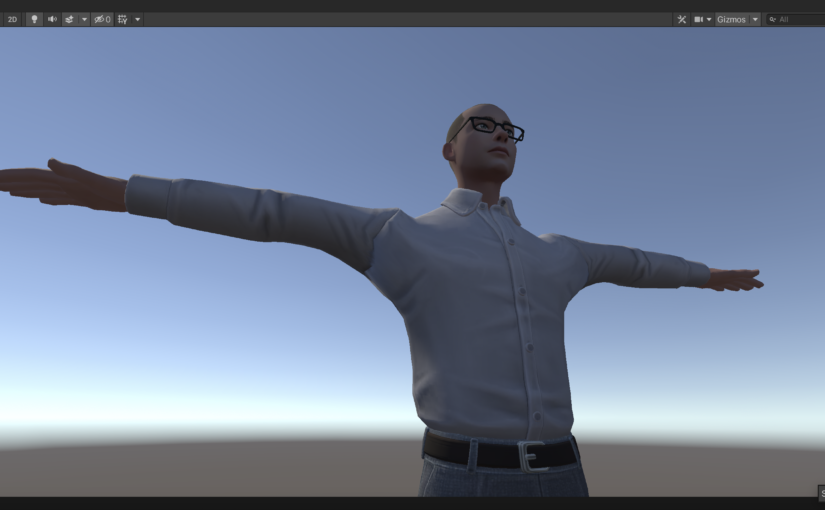
  20. Click on the model, then in the Inspector window, click on Rig. Choose Animation Type to be “Humanoid”. Click Apply.
  21. Staying in the Inspector window, click on Materials. Choose Material Creation Mode to be “Standard (Legacy)”, choose Location to be “Use External Materials (Legacy)”, and leave the other options at their defaults (Naming as “By Base Texture Name” and Search as “Recursive-Up”). Click Apply.
  22. Drag the model from Assets into the Scene.
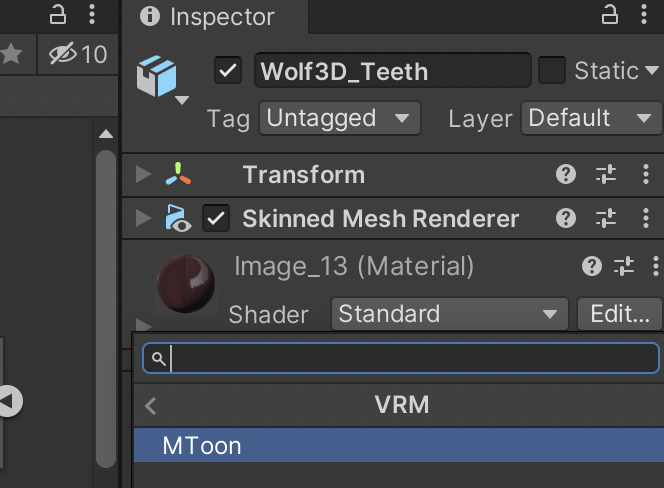
  23. If your model is meant to look like an anime figure, do this step, but otherwise (e.g. for more realistic avatars) skip it. Expand the newly created avatar in the Hierarchy window, and for each Material listed (which should be everything but Armature), click on it, then scroll down in the Inspector to the Shader. Click on the Shader drop-down (it may say something like “Standard”) and change it to VRM > MToon. Do this for all the materials in the model.
    Screenshot of Unity showing where to change the material Shader
  24. Alternatively, you can do other tweaks to the materials at this point. I find Unity makes the textures look a little grey, so this can be corrected by going into each Material as described in the previous step, opening up the Shader and changing the colour next to Albedo to use Hexadecimal FFFFFF (instead of CCCCCC). This is completely optional though.
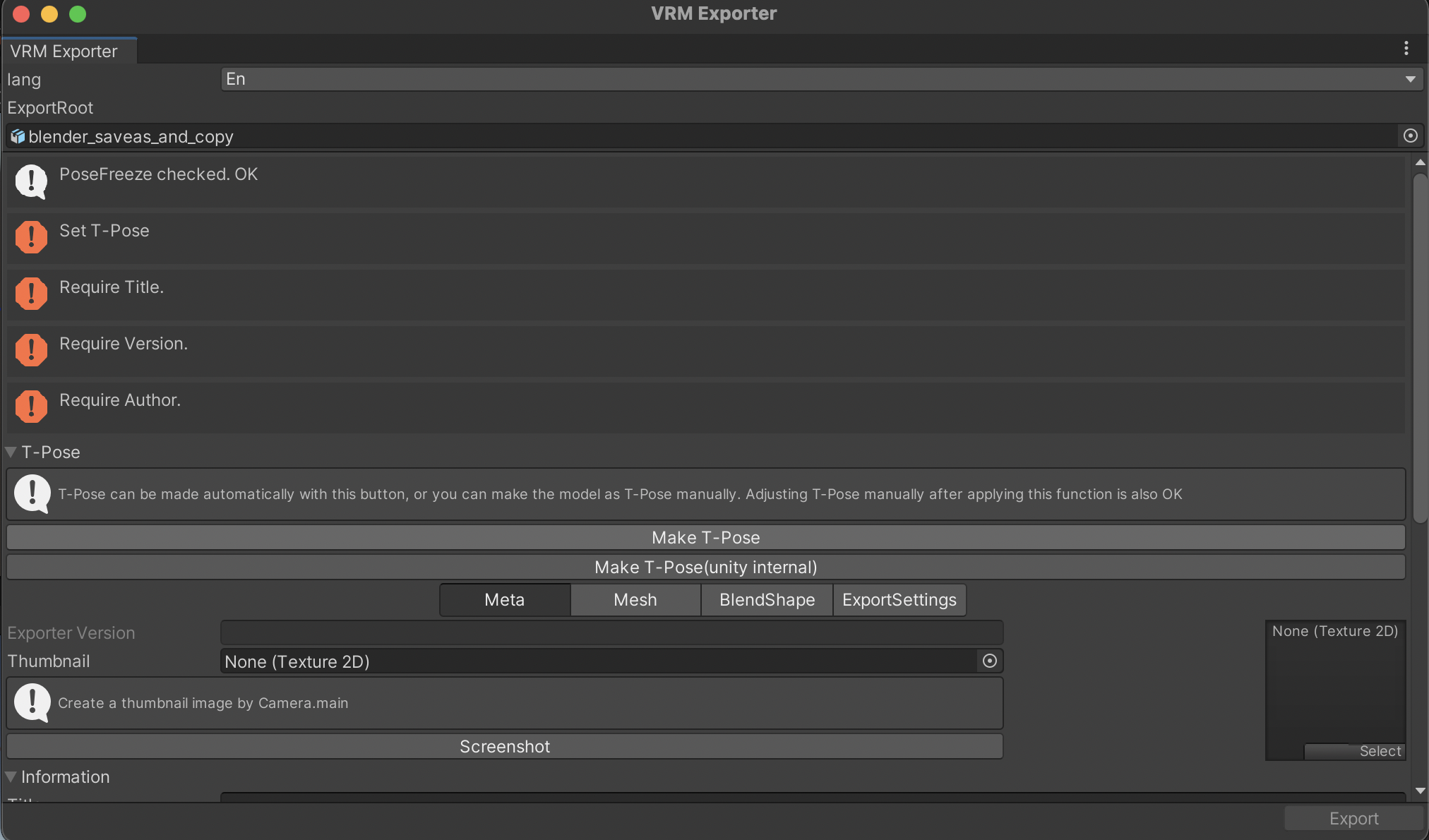
  25. Click on the avatar in the Hierarchy window, and then in the VRM0 top-level menu of Unity, select Export to VRM 0.x resulting in the export window popping up.
    Screenshot of Unity showing the VRM export window
  26. Click on “Make T-Pose”. Scroll down a bit and enter a Title (ie. the name of your avatar), a version (e.g. 1.0) and the Author (i.e. your name). Then click Export. Choose a name like “avatar” and save the VRM file into your vrm_assets folder.
  27. Delete the avatar that you just exported from the Scene by right-clicking it in the Hierarchy and choosing Delete. This just keeps the Scene neat for later.
  28. Now, drag the newly-saved VRM file into the Assets window of your Unity project. It is time to configure the lip synch and facial expressions.
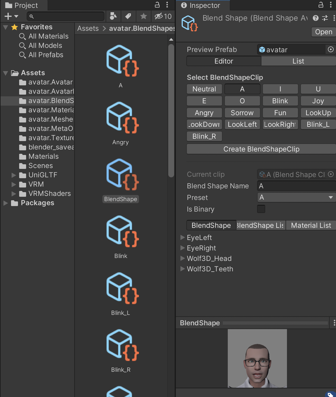
  29. Double-click on the BlendShapes asset (if you had saved the VRM file as avatar.vrm, this asset will be called avatar.BlendShapes) to show all the expressions that can be configured. Clicking on BlendShape will allow you to easily see and configure them in one place.
    Screenshot of Unity showing the configuration of Blend Shape
    Configuring the vowels will allow lip synch to work with your avatar, but you should configure all of it to ensure your avatar doesn’t look too wooden. Note that the vowels are in the Japanese order: A, I, U, E, O. Here are the settings that I used, but different avatars will need different values.
    • A:
      • Wolf3D_Head.viseme_aa 100
      • Wolf3D_Teeth.viseme_aa 100
    • I:
      • Wolf3D_Head.viseme_I 100
    • U:
      • Wolf3D_Head.viseme_U 100
    • E:
      • Wolf3D_Head.viseme_E 100
      • Wolf3D_Teeth.viseme_E 30
    • O:
      • Wolf3D_Head.viseme_O 100
      • Wolf3D_Teeth.viseme_O 100
      • Wolf3D_Teeth.mouthOpen 15
    • Blink:
      • Wolf3D_Head.eyesClosed 100
    • Joy:
      • Wolf3D_Head.mouthOpen 60
      • Wolf3D_Head.mouthSmile 48
      • Wolf3D_Head.browInnerUp 11
    • Angry:
      • Wolf3D_Head.mouthFrownLeft 65
      • Wolf3D_Head.mouthFrownRight 65
      • Wolf3D_Head.browDownLeft 20
      • Wolf3D_Head.browDownRight 20
    • Sorrow:
      • Wolf3D_Head.mouthOpen 60
      • Wolf3D_Head.mouthFrownLeft 50
      • Wolf3D_Head.mouthFrownRight 50
      • Wolf3D_Teeth.mouthOpen 30
    • Fun:
      • Wolf3D_Head.mouthSmile 50
    • LookUp:
      • EyeLeft.eyesLookUp 36
      • EyeRight.eyesLookUp 36
      • Wolf3D_Head.eyeLookUpLeft 75
      • Wolf3D_Head.eyeLookUpRight 75
    • LookDown:
      • EyeLeft.eyesLookDown 40
      • EyeRight.eyesLookDown 40
      • Wolf3D_Head.eyeLookDownLeft 20
      • Wolf3D_Head.eyeLookDownRight 20
    • LookLeft:
      • EyeLeft.eyeLookOutLeft 67
      • EyeRight.eyeLookInRight 41
    • LookRight:
      • EyeLeft.eyeLookInLeft 41
      • EyeRight.eyeLookOutRight 67
    • Blink_L:
      • Wolf3D_Head.eyeBlinkLeft 100
    • Blink_R:
      • Wolf3D_Head.eyeBlinkRight 100
  30. Now go back to the top level of the Assets window and scroll down to the avatar VRM model, then drag it into the Scene.
  31. Just as before, in the VRM0 top-level menu of Unity, select Export to VRM 0.x. You can leave the fields as they are, or update then. Click on Export. Save your VRM file into your vrm_assets folder with a new name to reflect it now has the expressions configured.
  32. Quit and save Unity, in case you want to come back and make further tweaks. You now have a VRM model.

Test out the VRM file in the avatar application of your choice! Good luck.

Gluten-free Pancakes Recipe

This is something I make regularly, and just like I previously recorded my Pancakes Recipe here, I’m recording my GF Pancakes Recipe here to make it easy to refer back to. It is originally based on Elizabeth Barbone’s excellent GF Pancakes Recipe.

Ingredients

  • 115g white rice flour
  • 60g corn flour
  • 60g sticky rice flour (a.k.a sweet rice flour a.k.a. glutinous rice flour)
  • 60g caster sugar
  • 15mL baking powder
  • 1/2 teaspoon table salt
  • 1/4 teaspoon xanthan gum
  • 2 large eggs
  • 1 cup (250mL) whole milk, or a little less
  • 1/4 cup (60mL) vegetable oil, or similar, e.g. canola oil
  • 1 teaspoon vanilla extract

Method

  1. Sift all the dry ingredients (flours, sugar, salt, baking powder and xanthan gum) into a mixing bowl, and stir with a fork to combine.
  2. Crack the eggs into a glass, stir with a fork, and add to the mixing bowl, together with half (!) the milk, and all the other wet ingredients. Stir with a fork to make a thick mixture, and keep stirring briskly until it is smooth.
  3. Gradually add more milk, stirring each time, until the batter pours smoothly, and is the consistency of a milkshake. You may not need all of the milk.
  4. Heat up a flat frying pan on a low-to-medium heat, and spread with a little butter. It should sizzle when hot enough. Don’t let it get so hot that the butter burns.
  5. Use a 1/4 cup measure to scoop the pancake batter onto the frying pan. I use silicon egg rings to help form the pancakes into a consistent round shape. When bubbles just start to form on the top, I remove the rings and gently flip the pancakes, and cook until it is browned on both sides.
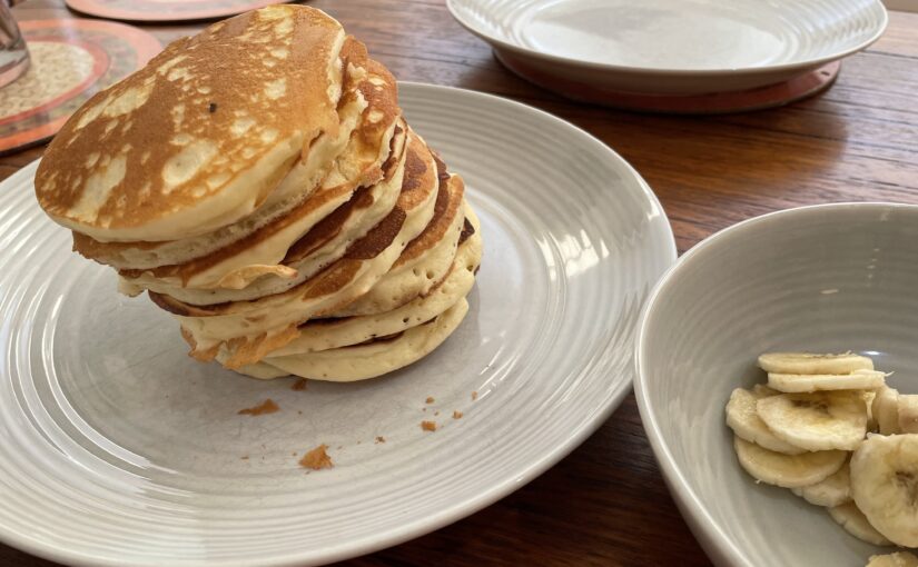
  6. If you keep them in a stack as you take them out of the frying pan, they tend to stay warm longer. That is, if they aren’t immediately eaten.
  7. Serve with maple syrup and sliced banana, or whatever takes your fancy!

Makes about 10 pancakes.

Turning up for work as an avatar

I don’t think we’re talking enough about avatars. I don’t mean the James Cameron film or the classic anime series. I’m referring to the computer 3D model that can represent you online, instead of a picture or video of the “real you”.

Due to the Covid-19 pandemic, we’ve had something like 5 years of technology uptake in an accelerated timeframe. Remote working has become much more common, with people regularly joining meetings with colleagues or stakeholders via services like Teams, Webex or Zoom rather than meeting up in person.

While pointing a camera at your face and also seeing an array of boxes containing other people’s faces has its merits, it can have a bunch of downsides. It turns out that many of these can be addressed by attending the meeting as an avatar rather via camera.

Interacting with others via avatars is the normal way of things when it comes to computer games. Many people are familiar with avatars from online social settings like Minecraft, Fortnite or Roblox. I’d think that for many kids today, they have spent more hours interacting online with others as an avatar than on camera.

So, it may be there is a generational shift coming as such people come up through our Universities and workplaces. But there are also fair reasons for moving to use avatars for meetings in any case. Here are five reasons why you should consider turning up for work online as an avatar.

1. It’s less stress

Being on camera can be a bit stressful, since your appearance is broadcast to all the other people in the same meeting, and other people can be a bit judgy. Why should your appearance be the concern of people that don’t need to share the same physical space as you?

If you attend a meeting as an avatar, you

  • Don’t have to shave, brush hair, put on makeup
  • Don’t have to worry about a pimple outbreak, or a bad haircut
  • Don’t have to get out of pyjamas, take off a beanie, or cover up a tattoo
  • Know there’s no chance of someone embarrassing wandering past in the background or a pet leaping up in front of you

2. You will appear more engaged

Well, if having the camera on is stressful, why not just turn it off? In some workplaces or schools, it is considered bad etiquette to turn off your camera in a group video call. It is not a great experience to be talking to a screen of black boxes and not seeing anything of your audience. Seeing a participant’s avatar watching back instead of a black box is a definite improvement.

However, sometimes it is a good idea to turn off the camera, such as when eating or having to visit the bathroom. The participant is still engaged in the meeting but for good reasons has turned off the camera. There is no need to do that with an avatar.

An avatar is also able to make eye contact through the meeting. Unfortunately, not everyone with a camera can do this, as the camera position might be to the side, above or below the screen that the participant is actually looking at. This tends to make the participant look distracted, as that would be how such behaviour would be interpreted in a face-to-face meeting. Avatars don’t have this issue.

3. Avatars are more fun

With Teams, Webex or Zoom, you can replace your background with a virtual background for a bit of fun. With an avatar, you can change everything about your look, and make these changes throughout the day.

You don’t even need to be human, or even a living creature. You might want to stick to an avatar that is at least humanoid and has a face, but there’s a huge creative space to work within.

In some online services, avatars are not limited to being displayed in a box (like your camera feed is), but can interact in a 3D space with other avatars. This also means that stereo audio can be used to help position the avatar in a physical space, making it easier to tell who is speaking by just where the sound is coming from, or distinguish a speaker when someone is talking over the top of them.

4. There may be less risk of health issues

Most group video meeting services show a live feed of your own camera during the call. It’s not exactly natural to spend hours of a day looking at yourself in a mirror, especially if the picture of you is (most likely) badly lit, from an odd or unflattering angle, and with a cheap camera lens. Then, if you couple this with seeing amazing pictures of others online, say on social media, it all appears to be a bit unhealthy.

While it’s not an official condition, there is some discussion about what is being called Zoom dysmorphia, where people struggle to cope due to anxiety about how they appear online. These people may go the plastic surgery route in order to deal with this.

Having a camera on all the time may also be generally unhealthy since it ties people to the desk for the duration of the call. Without this, for some meetings, people might instead take a call while walking the dog or taking a stroll around the block.

5. It works well for hybrid meetings

Hybrid is hard. It’s typically not a level playing field to have some meeting participants together in a room and some joining remotely. Having a camera at the front of a room capturing all of the in-person attendees means it is often difficult for the remote participants to see them.

The main alternative is that all the participants in the room have a device in front of them that allows them to join the meeting as a bunch of remote participants who happen to be in the same place. This usually results in a bunch of cameras pointing up people’s noses, as the cameras in a laptop or tablet are not at eye-level.

If the people in the room join as avatars, they can be showed nicely to the other participants, and the individuals’ cameras are often still adequate for animating their avatar to track with their face and body.

However

There are some down-sides to using avatars. It can make it more difficult for hard-of-hearing participants since they can’t rely on lip reading to follow a conversation. There will need to be avatar etiquette discussions so people aren’t made uncomfortable by certain types of avatar turning up to meetings. The technology is still evolving so it can look a bit unnerving if an avatar doesn’t show expected human emotions.

But directionally, avatars solve problems with our current group video meetings, and we can expect to see them become more mainstream over the coming years.

What is a qubit?

I am not a deep expert in quantum computing, but I know several who are. In order to chat to them, I have read quite a few introductory quantum computing articles or online courses. However, I find that these are either pitched at a level where it’s all about the hype, or at a level where you need to have a good background in either mathematics or physics to follow along. So, I have been trying to describe a quantum computer in a useful way to people without the technical background.

This is just such an attempt. If you’re still with me, I hope you find this useful. This is for people that don’t know the difference between Hamiltonians, Hermitians or Hilbert spaces, and aren’t planning to learn.

Let’s start with some definitions. A quantum computer is a type of computing machine that uses qubits to perform its calculations. But this raises the question of what is a qubit?

Digital, or classical, computers use bits to perform their calculations. They run software (applications, operating systems, etc.) that run on hardware (CPUs, disk drives, etc.) that are based on bits, which can be either 0 or 1. The hardware implementation of these bits might be based on magnetised dots on plastic tape, pulses of light, electric current on a wire, or many others.

Qubits are “quantum bits”, and also have a variety of hardware implementations such as photon polarisation, electron spin, or again many others. Any quantum mechanical system that can be in two distinct states might be used to implement a qubit. We can exploit the properties of quantum physics to allow a quantum computer to perform calculations on qubits that aren’t possible on bits.

Before we get to that, it is worth noting that quantum computers are known to be able to perform certain calculations in minutes that even a powerful classical computer could not complete in thousands of years. For these specialised calculations, the incredible speed-up in processing time is why quantum computers are so promising. As a result, quantum computers look to revolutionise many fields from materials engineering to cyber security.

Since a qubit can be made from a variety of two-state quantum systems, let’s consider an analogy where we implement a qubit on something we all have experience with: a coin. (I know this is not an exact analogy since a coin is a classical system not a quantum mechanical system, and it can’t actually implement entanglement or complex amplitudes, but it’s just an analogy so I’m not worried.)

If we consider a coin lying on a table, it can be either heads-up or heads-down (also known as tails). For the purposes of this analogy, let’s call these states 1 and 0. You will recognise that this is like a classical bit.

Maybe this coin has different types of metals on each side, so we could send some kind of electromagnetic pulse at it to cause it to flip over, and this way we could change it from 1 to 0, or visa versa. If there is another coin next to it, we might consider another kind of electromagnetic pulse that reflects off only one of those metals in a way that would flip the adjacent coin if the first coin’s 1 side was up. You might ultimately be able to build a digital computer of sorts on these bits. (You can build a working digital computer within the game of Minecraft, so anything’s possible.)

Let’s now expand our analogy and add a coin flipping robot arm. It is calibrated to send a coin up into the air and land it on the table, such that it always lands with the 0 side up. While the coins are in the air, these are our qubits. When they land on the table, they become bits.

Now we can flip coins into the air, and send electromagnetic pulses at them to change their state. However, unlike bits that can be only either 0 or 1, qubits have probabilities. A pulse at a coin can send it spinning quickly so that when it lands on the table it will be either 0 or 1 with a 50-50 chance. Another pulse might reflect off this spinning coin so that it hits the next coin and spins it only if the pulse happens to hit the 1 side of the first coin. Now when the coins land, they have a 50-50 chance of either being both 0 or both 1.

However, you won’t know this from measuring it just the one time. You will want to perform the coin flips and the same electromagnetic pulses a hundred times or more and measure the number of different results you get. If you do the experiment 200 times, and 100 of those times you get two 0s and the other 100 times you get two 1s, you can be pretty confident that this is what is going on. For more complicated arrangements of pulses, and greater numbers of coins, you might want to do the experiment 1000 times to have a clear idea of what is happening.

This is how quantum computing works. You perform manipulations on qubits (coins in the air), these set up different possible results with different probabilities, the qubits become bits (coins on the table) that can then be read and manipulated by a classical computer, and you repeat it all many times so you can determine things about those probabilities.

Gluten-free Donuts (or Doughnuts)

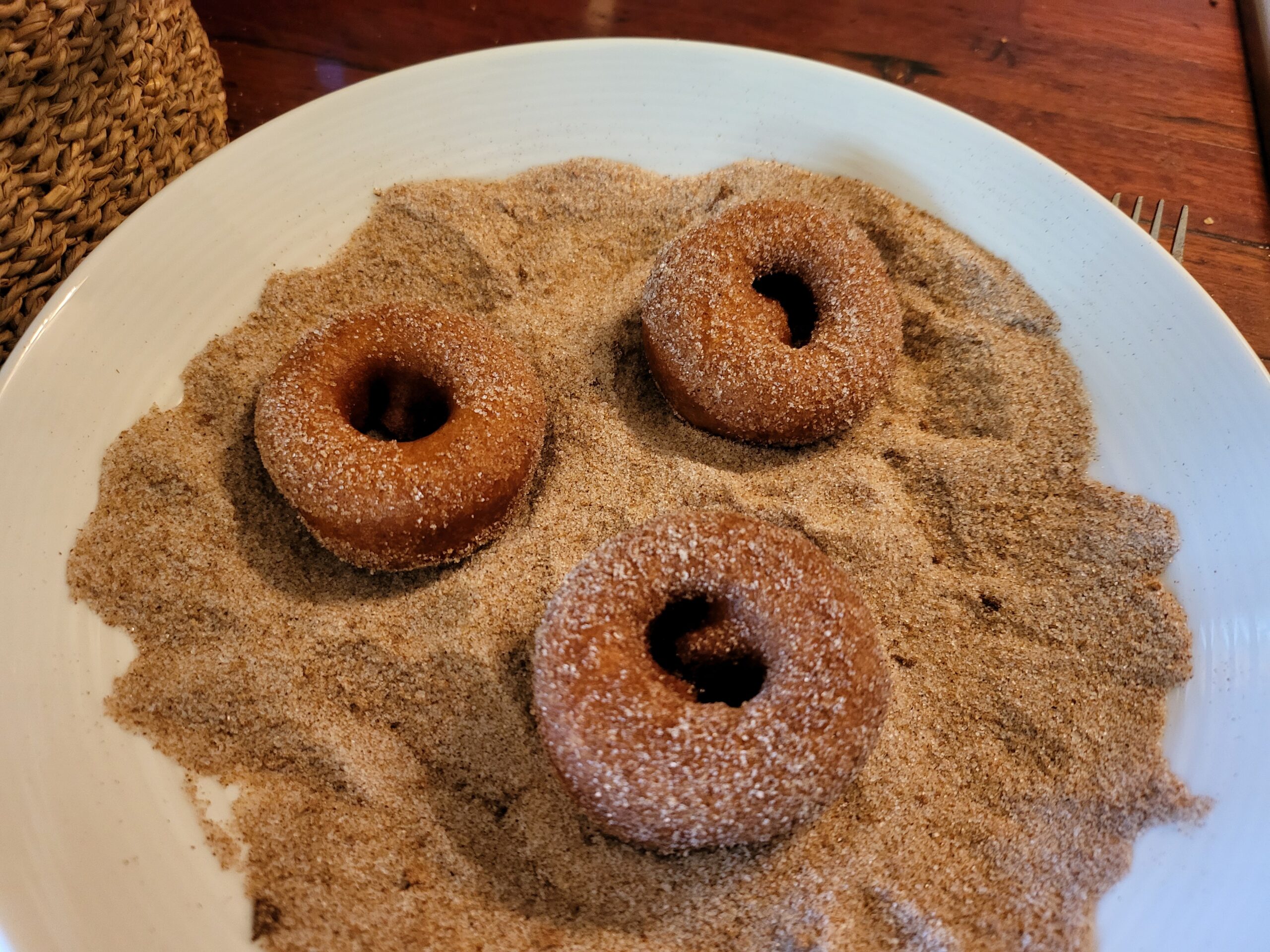
I like ’em, whether they are called donuts or doughnuts, especially when they are fried, ring-shaped, and covered with a cinnamon-and-sugar powder. I recently impulse-bought a donut maker – one of the kinds that drops rings of batter into hot oil – and was looking forward to making some of my favourite kind.

However, when I went to search for a gluten-free, fried ring donut recipe, I couldn’t actually find one. I checked my trusty gluten-free recipe books and did several versions of web searches, but I didn’t find what I was looking for. I did discover some interesting yeasted donut recipes that I have put aside to try another time, though.

So, after a bit of experimentation, here is my recipe for gluten-free, fried ring donuts. It was based on this recipe for gluten-and-dairy free donuts that was pretty similar to the (glutinous) one on the box of the donut maker, but was for oven-baked donuts rather than fried ones.

Before you begin

bottom outlet of a plastic donut maker showing the rod centred in the middle of the outlet

It is important to ensure your donut maker is going to work for you. Perhaps I can’t be too fussy about a $13 donut maker, but it still needs to work. After it arrived, mine needed to be gently adjusted by pushing the internal component to re-seat itself in the plastic channels. Also, the plastic rod was a little warped, so when I pressed down on the top of the donut maker, the plastic rod – that ultimately forms the “hole” in the final donut – wasn’t centred correctly. I needed to spin the rod in place until when I pressed the button at the top, the rod stayed centred in the circular outlet at the bottom of the donut maker. I then used a permanent marker on the button at the top of the rod and the outer rim of the donut maker to help show me where it needed to stay aligned to for a good donut shape to be created.

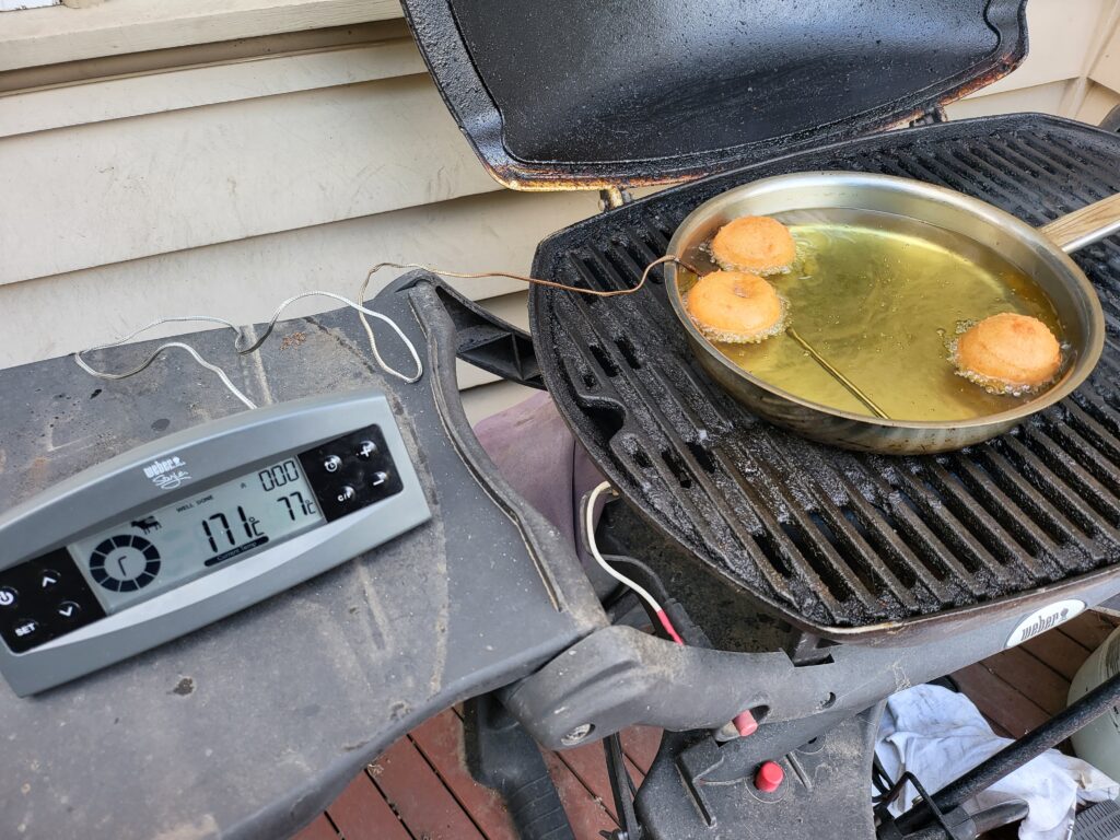
three donuts in a frypan on a bbq with a bbq thermometer reading the oil temperature as 171 degrees Celcius

You also want to be able to control your oil temperature. For me, I used a BBQ thermometer and heated the oil in a frypan outside (to keep the hot oil smell out of the house). I could then control the oil temperature by either raising/lowering the lid of the BBQ or adjusting the gas setting. Around 180 degrees Celcius is the best temperature to fry your donuts, so ensure you can manage that +/- 10 degrees. A thermometer of some kind is highly recommended!

Ingredients

  • 140 g of gluten-free plain flour (a type with no xanthan gum)
  • 1/2 teaspoon (2.5 mL) of xanthan gum
  • 1 teaspoon (5 mL) of gluten-free baking powder
  • 1/2 teaspoon (2.5 mL) of table salt
  • 50 g of caster sugar
  • 1 teaspoon (5 mL) of ground cinnamon
  • 1 large egg
  • 1 teaspoon (5 mL) of vanilla extract
  • 80 mL of canola (or vegetable) oil
  • 175 mL of milk
  • 1 teaspoon (5 mL) of vinegar
  • At least 1 L of canola oil, or other suitable oil, for frying
  • Extra caster sugar and ground cinnamon for coating

Method

  1. Heat up the oil for frying, but keep an eye on it that it doesn’t get too hot.
  2. Sieve the dry ingredients into a large mixing bowl, and then combine well with a fork.
  3. Lightly beat the egg, and then add it and the other wet ingredients into the same mixing bowl. Beat until smooth, and then scrape into the donut maker.
  4. When oil is at temperature (near to 180 degrees Celcius), begin using the donut maker. Hold it just above the oil and press down on the button. The mix will be quite thick, but gently shake the donut maker and after about 5 seconds, there should be a good quantity of donut mix held at the end of the donut maker. Release the button and it should cut the mix away from the donut maker to drop a nicely-shaped ring of batter into the hot oil. Cook a batch of donuts together, maybe 3 or 4, or more depending on the size of your frypan or pot.
  5. Let the donuts cook for a couple of minutes, and then using a slotted metal spoon (or a potato masher in my case), gently turn the donuts over to cook for a couple more minutes. When they are done they should be a dark golden colour.
  6. Remove the batch of donuts to a plate covered with paper towel, allowing you to start another batch of donuts.
  7. Toss the cooked donuts in a mix of caster sugar and cinnamon (maybe 1 teaspoon of cinnamon to 50 g of caster sugar, but do whatever you feel tastes best), and then move to a cooling rack or plate.
  8. As with most gluten-free baking, these donuts will taste best when you’ve allowed them to cool to room temperature. It can be very tempting to eat them while they are still warm, but they will taste like they are undercooked at that point, sorry.

Makes 20 or so 6 cm-diameter donuts.