This is the first in a series of four articles based on my Jupyter Notebooks exploring quantum computing as a tool for generating random number distributions.
Many of the introductory quantum computing articles and courses out there are not quite right. They either quickly head deep into details that require a University-level physics or mathematics background, or sit at a high level based on analogies that are out of step with how quantum computers actually work. I want to try something different, and introduce some useful quantum computing algorithms using high-school level maths. I will avoid much (but maybe not all) of the jargon, and show how the algorithms can be implemented on the commonly available Qiskit platform.
In my earlier article on quantum computing, I introduced an analogy to describe quantum computers, which are based on qubits rather than bits. The analogy was of a coin-flipping robot arm that is flipping a coin that lands on a table. A qubit is like the coin when it is in the air, and a bit is like the coin when it has ended up on the table. When it’s in the air, the coin is in a kind of probabilistic state where it may end up heads or tails, but once it’s on the table, it’s in a certain state where it is definitely one of either heads or tails. Quantum computers work in the realm of probabilities, and can manipulate the coin while it’s still spinning in the air. The spinning coin in the air is the qubit. But at some point it will land on the table and be measured as either heads or tails. At that point it becomes a bit.
To write about quantum states, a notation is used where the name of the state is put between a vertical bar and an angle bracket. Just like a single bit can be in the “0” state or the “1” state, for a single qubit, we might say it can be in the |0> state or the |1> state. Our hypothetical robot-arm is well-calibrated, so it consistently flips a coin that lands with the same side facing up, and the resulting coin is like having a qubit in one of these states. The coin is in a probabilistic state, but the probability of it having a particular result is 100%. Similarly, if a qubit is in the |0> state, when it is measured, you will get a “0” result 100% of the time.
However, a quantum computer can manipulate the probabilities of the qubit, so even if the qubit started in the |0> state, after manipulation it enters a new state where if the qubit is measured, it will get “0” outcome 50% of the time (and “1” outcome the other 50% of the time, of course). This is done using a Hadamard operation, usually just written as H. We will use this operation to create truly random numbers.
Creating truly random numbers
Mostly when you have a computer give you a random number, such as using the RAND function in Microsoft Excel or when you’re playing a computer game and the enemy does something unexpected, the computer is actually producing a pseudo-random number. If you could create a perfect snapshot of everything in your computer, then get it to do something “random”, and return to that snapshot again, it will do exactly the same random thing each time. So, it’s not actually random, but it looks random unless you peer too closely.
For most applications, that’s fine. But if you are doing cryptography, having truly random numbers is important. You want to generate a secret key that no-one else can guess. Ideally, even if someone could take a snapshot of your computer, they still couldn’t predict what secret key is generated. There are special hardware random number generators that can create truly random numbers (Cloudflare uses lava lamps!), and quantum computers create truly random numbers too.
Let’s say we are going to generate a 2 bit random number. We’ll use 2 qubits, and the starting state of the qubits will be |00>, which means the outcome of measuring them both as “0” is 100%. We’ll use a quantum computer to manipulate the qubits so that all four possible outcomes |00>, |01>, |10>, or |11> are equally likely. Then when the qubits are measured, we will have some truly random bits.
We can write the four possibilities as a vector, with each row consisting of the probability of that outcome. Quantum computers perform their calculations using complex numbers rather than real numbers, and this is because complex numbers are needed to accurately describe how things work at the quantum level. We can simplify things, and just use real numbers, but we will need to calculate probabilities by squaring the values in each row of the vector.
We call this vector the quantum state vector (or just state vector), and it starts with being
$$\begin{bmatrix}
1.0 \\
0.0 \\
0.0 \\
0.0
\end{bmatrix}$$
Each row of the state vector corresponds to a different outcome, with the outcomes for two qubits being |00>, |01>, |10>, and |11> as we go down the vector. So this state vector represents a 100% probability of getting the |00> outcome.
We want each outcome to have a 25% probability, so we want to change the state vector to be:
$$\begin{bmatrix}
\frac{1}{2} \\
\frac{1}{2} \\
\frac{1}{2} \\
\frac{1}{2}
\end{bmatrix}$$
Of course, when you square 1/2, you get 1/4, or 25%.
The H operation is a standard operation on quantum computers, and works on all pairs of rows of the quantum state vector where that outcome differs only by the value of a specific qubit, e.g. where one outcome has the |0> for that qubit and the other row has |1>. For each pair, it turns the first value into a new value that is the sum of the original values divided by \(\sqrt{2}\), and the second value into the difference between the original values divided by \(\sqrt{2}\). While it is a division by \(\sqrt{2}\) rather than a division by 2, you can think of H like a “half” operation, where it calculates half the sum and half the difference and is scaled by a normalisation constant so that when the values are squared, the probabilities add up to 1.0. Written out mathematically, if the first row value is \(a\) and the second row value is \(b\), the first row value becomes \(\frac{a+b}{\sqrt{2}}\) and the second row value becomes \(\frac{a-b}{\sqrt{2}}\).
To get the desired final state vector from the initial state vector, we can apply H first to the pair of rows associated with a difference in the right-most qubit, then apply H to the pair of rows associated with a difference in the left-most qubit. Here’s how it would go:
| Qubits | Initial state vector | Working out first H | Result of first H | Working out second H | Result of second H |
|---|---|---|---|---|---|
| |00> | 1.0 | =\(\frac{1.0+0.0}{\sqrt{2}}\) | \(\frac{1}{\sqrt{2}}\) | =\(\frac{\frac{1}{\sqrt{2}}+0.0}{\sqrt{2}}\) | \(\frac{1}{2}\) |
| |01> | 0.0 | =\(\frac{1.0-0.0}{\sqrt{2}}\) | \(\frac{1}{\sqrt{2}}\) | =\(\frac{\frac{1}{\sqrt{2}}-0.0}{\sqrt{2}}\) | \(\frac{1}{2}\) |
| |10> | 0.0 | =\(\frac{0.0+0.0}{\sqrt{2}}\) | 0.0 | =\(\frac{\frac{1}{\sqrt{2}}+0.0}{\sqrt{2}}\) | \(\frac{1}{2}\) |
| |11> | 0.0 | =\(\frac{0.0-0.0}{\sqrt{2}}\) | 0.0 | =\(\frac{\frac{1}{\sqrt{2}}-0.0}{\sqrt{2}}\) | \(\frac{1}{2}\) |
Now that we’ve covered the process, let’s look at how this would be written programmatically using the Qiskit library from IBM.
Implementing this on Qiskit
We’re going to set up a (simulated) quantum computer with 2 qubits. (You can grab the complete Python script from here, or just type in the code below.)
import numpy as np
from qiskit import QuantumCircuit, QuantumRegister, ClassicalRegister, execute, BasicAer
from qiskit.quantum_info import Statevector
from qiskit.visualization import plot_histogram
import matplotlib.pyplot as plt
backend = BasicAer.get_backend('qasm_simulator')

q = QuantumRegister(2)   # We want to use 2 qubits
algo = QuantumCircuit(q) # Readies us to construct an algorithm to run on the quantum computer
By convention, all qubits begin in the lowest-energy state, so without doing anything, the qubits of our quantum computer should be set to |00>. We can check the state vector and see.
v1 = Statevector(algo)
print(np.real_if_close(v1.data))
Which will print “[1. 0. 0. 0.]” and shows the |00> row is 1.0 and the other possible outcomes are 0.0.
Qiskit numbers the right-most qubit as qubit 0, and the one to the left of it as qubit 1, with the next as qubit 2, and so on. You may have come across this as being called little-endian. Let’s start by using the H operator on pairs of rows associated with the |0> and |1> outcomes on qubit 0 (the right-most qubit).
algo.h(0)  # Apply H operation on pairs of rows related to qubit 0
v2 = Statevector(algo)
print(np.real_if_close(v2.data))
Which will print “[0.70710678 0.70710678 0. 0. ]”, and given 0.70710678 is \(\frac{1}{\sqrt{2}}\), it is what we were expecting. Now to do the H operation on the pairs of rows associated with the other qubit (qubit 1).
algo.h(1)  # Apply H operation on pairs of rows related to qubit 1
v3 = Statevector(algo)
print(np.real_if_close(v3.data))
Which will print “[0.5 0.5 0.5 0.5]”. The application of the H operations has set up the state vector so that the quantum computer should give us different randomly generated 2 bit values with uniform distribution. Let’s add a measurement to the end of our algorithm, and have the quantum computer do this 1,000 times and see what we get.
algo.measure_all()  # Measure the qubits and get some bits
result = execute(algo, backend, shots=1000).result()  # Run this all 1,000 times
plot_histogram(result.get_counts(algo))
plt.show()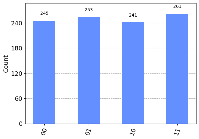
This shows that of the 1,000 times this was performed (1,000 “shots”), the different 2-bit results occurred approximately the same number of times. It is what you would expect of a uniform distribution, noting that it is unlikely for every possibility to occur exactly the same number of times.
You can extend this process to as many random bits as you want, by having a qubit for each and applying the H operation in turn for each qubit. Quantum computers are still not very big, so you’ll run out of available qubits quickly. Or, you may want to just to re-run this process and get another two random bits each time.
We used a quantum computer simulator here, so it’s still a pseudo-random result. To use an actual quantum computer, you would need to set up an account on IBM Quantum, get an API key, and change the backend to point at an instance of a quantum computer from their cloud. This is easy enough to do, but is an unnecessarily complication for this article.
You can then access true random bits that can be fed into any software that needs it. With all that, you have seen how to create a simple quantum algorithm and make it do something useful that is not easily done on a digital computer.
Please let me know… Were you able to follow this description of quantum computation? Do you feel confident that you could get this working on a real quantum computer? Would you prefer if there was more linear algebra, matrices and complex numbers in this article?